The relationship between the short run and the long run

First off, we're going to talk about tangency.

LEFT OF TANGENCY: This is when there is too much capital to efficiently produce a specific quantity of output. In other words, the SRAC > LRAC. This can be corrected by subletting capital (hence moving us into the long run)

Eg: You want to produce 20 letters. You have 3 meters of office space, and two secrataries who each produce 10 letters. Each secratary only requires 1 meter of office space though, so there is an extra meter of office space which is adding an unecessary burden to your overhead costs.

AT TANGENCY: This is when there is exactly the right amount of capital to efficiently produce a given quantity of product. In other words, the SRAC = LRAC. You don't need to change anything, because production is already the most efficient it can be for that level of output.

Eg: You want to produce 20 lettters. You have 2 meters of office space, and two secrataries who each produce 10 letters. Each secratary only requires 1 meter of office space, so this is perfect. There is just the right amount of secrataries and office space to produce 20 letters.

RIGHT OF TANGENCY: This is when there is too little capital to efficiently produce a specific quantity of output. In other words, the SRAC > LRAC. This can be corrected by purchasing capital (hence moving us into the long run)

Eg: You want to produce 30 letters. You have 2 meters of office space, and 3 secrataries who each produce 10 letters. Each secratary requires 1 meter of office space though, so there isn't enough office space for each secratary to do her job most efficiently.

What we can see here is that LRAC is an 'envelope' of all SRAC curves. Each point on the LRAC curve represents a tangency point with a short run cost curve for a different amount of capital. This tangency point is the OPTIMAL level of fixed factor of each output level.

So basically, each different short run cost curve tangent to the long run cost curve represents a different level of capital.

NOTE there is only one point of the entire LRAC curve where the SRAC curve is tangent to the LRAC at it's minimum.

IT IS ALWAYS MORE EFFICIENT FOR FIRMS TO HAVE LOWER COSTS. USUALLY, THIS MEANS BEING TANGENT TO THE LRAC CURVE!

--------------------
Deriving the supply curve:

SR:
-One Fixed Factor
-Fixed Prices

LR:
-All Factors Can Vary
-Prices Can Also Vary

Demand can increase independently from supply. As we know, an increase in demand leads to an increase in the price. An increased unit price for products will generate positive economic profits for producers in high-demand industries. This acts as a signal for other firms to enter this industry. As a result, the overall supply for this product will increase.

The long run supply is a conjoined trail of all the points on intersection caused by demand induced shifts in short run supply (thus, the long run supply is not always necessarily upward-sloping).

Long run supply may increase, remain constant, or decease depending factor price changes and the conditions of entry into that particular industry.

The long run average costs for each firm SHIFTS as the industry expands.

Economies of scale determine the shape of the long run average cost curve
Shifts in the long run average cost determine the shape of long run supply

Cost Curves-Econ 101

Econ 101- The introduction of the cost curve!

Last lecture, we studied the production curve, and learned about the law of diminishing marginal productivity- basically, that after a certain point (the inflection point), adding more variable factor (ie labour) will causes the marginal productivity to decrease.

Today, we're going to look at full cost curves, and discover how to derive them from the product curve.

It includes several factors:
Total Costs
Total Fixed Costs (overhead costs like rent, licenses and insurance: these do not change with quantity produced)
Total Variable Costs (costs like wages, supplies, etc. which change with the quantity produced)

Average Variable Costs: TVC/Q
Average Fixed Costs: TFC/Q
Average Total Costs: TC/Q
Remeber: Average costs are always a ray from the origin on the total cost curve.

Marginal Fixed Costs (Always zero)
Marginal Variable Costs: /\Total Variable Costs / /\Quantity Supplied
Total Variable Costs: /\Total Costs / /\Quantity Supplied
Remember: Marginal costs are always the slope of the derivative of the same point on the total cost curve.

Cost curves use the following formulas:

Total Costs = f(Q produced)

Total Costs = Total Variable Costs + Total Fixed Costs

Average Total Costs = Average Fixed Costs + Average Variable Costs.

TOTAL FIXED COSTS

These don't change as production increases, so the cost is constant throughout production

AVERAGE FIXED COSTS

These fall as production increases. This is called spreading overhead costs. Each additional unit produced has to cover a smaller and smaller portion of the original overhead costs.


TOTAL VARIABLE COSTS

The shape is due to specialization and saturation. Basically, remembering the production curve, we know that production initially increases at an increasing rate due to specialization and division of labour. This means that due to increased efficiency, the variable costs will not rise significantly for a particular range of output (because no new workers will be required to meet these production targets, so no extra wages will have to be paid).

As saturation occurs, we require more and more workers to be working to produce higher quantities of product. This causes our costs to rise, because each additional worker must be paid wages. Basically, we can infer that all of the cost changes seen on the variable cost curve are the result of production changes seen on the short run production curve.

AVERAGE VARIABLE COSTS

Similar to average production, only flipped upside down!

TOTAL COSTS-combining the two

As you can see, the average cost curve and the marginal cost curve are the rays and derivatives from the total cost curve.

The average cost and marginal cost curves are valley-shaped for the same reason that the average and marginal production curves are hill-shaped. When a firm is at capacity, it's average cost valley is at its lower point, and it's average producttion hill is at it's highet point.

Marginal costs intersects both the average costs and the average variable costs at their minimums.

AC is cup shaped
AVC is saucer shaped (they are lower than average costs because average costs also include average fixed costs)
MC is spoon shaped

PRODUCTION AND COST CURVES ARE VERY CLOSELY LINKED- costs are closely linked to production realities

There are two things which can shift the cost curve:

1: a change in input prices (varies directly with the cost curve. For an example, if I run a furniture factory, and the price of lumber goes up, my costs will all rise)

2: a change in fixed factor (this is a long-run planning decision), which can benefit or harm a firm, depending on production realities. Will a bigger lumber factory decrease average costs? It depends on how production goes- all we need to know is that it DOES change things!

Introduction to cost curves!

Okay! Last lecture was all about firms. Now today, we're gonna talk about how we derive the Short-run supply curve. We must examine the theoretical link between price and quantity produced!

Price --------> [?]----> Quantity Supplied

What is the missing link???
PROFITS!!!!

We assume, as economists that producers (like consumers) want to be as happy as possible. Instead of maximizing utility, however, consumers are made the most happy by maximizing total profits!

Total profits = total revenue - total costs

TOTAL REVENUE
-total revenue = price X quantity
-Total revenue is changes based on different kinds of markets (there are different revenue curves for markets with perfect competition, imperfect competition, and monopolies. We talk about all of these in the upcoming chapters!)

TOTAL COSTS on the other hand are the same for each market structure. We're gonna talk about total costs in this chapter!

OKAY! Let's think about production! What is production?

Well... production is the transformation of various inputs into outputs, which is performed by a firm. For an example, when joe the employee, rent for a smoothie shop, electricity, a blender, yoghurt, mangoes, and bananas are used together to create a mango-banana smoothie, THAT is production.

INPUTS are the factors of production (factors)
OUTPUTS are goods and services (commodities)

There are 5 factors of production

Capital- (Plant or Factory, Equipment, Inventory, and Residential Inputs)
Land- Natural Resources
Labour- Human Resources (Employees)
Technology- Changes and innovations in the production process
Entrepreneurship- Innovation, Invention, Research and Development (new and exciting ideas)

THE PRODUCTION FUNCTION: Maximum output is a function of inputs

For the sake of simplicity, we focus on the relationship between 2 inputs: Capital and Labour.
TP = f (Labour, Capitol)

Let's say we've got an office where we produce written letters using secrataries. The number of letters written is a function of the office infrastructure and the number of secrataries employed.

COSTS: The value of the factor used up in production (the value of inputs)
REMEMBER: Opportunity costs determine decision-making in the firm (inputs are valued depending on their next best allocation, not their sticker-price). We call the costs with ppportunity cost factored in the IMPUTED OR IMPLIED COST (OR IN GATEMAN'S LECTURES, THE OPPORTUNITY COST).

The Accounting Cost is not something we look at in Economics. It is used in business school, and merely includes the explicit invoice prices of factors. It does not take the owner's time and money, for example, into consideration.

SUNK COSTS, however, are not factored in to opportunity cost, because they have no alternative use (or salvage value). In other words, they have No 'next best' allocation. An example of a sunk cost would be a computer program which is designed and purhcased specifically for your business. This input cannot be used any other way, so Opportunity cost is 0, and it is a sunk cost!

PROFITS!

ACCOUNTING PROFIT = total revenue - Accounting costs (the sticker prices of inputs). This does not include opportunity costs.

ECONOMIC PROFIT = Total Revenue - Total Costs (and includes opportunity costs). This is also known as pure profit, supra-normal profit, or in an econmics class, simply 'profit'. It basically measures profit compared to other opportunities. In order to understand economic profit, it is important to understand the idea of normal profit.

NORMAL PROFIT is actually a cost. It is the cost of technology and entreprenuership, or the implicit cost of risk taking. It is the cost of choosing to devote time and money into a certain business instead of simply putting money in the bank or working at the next-most-profitable business. For an example, if I can make 5% returns on my money in the bank, then those 5% returns are considered normal profit, and should be added to my economic costs. In the long run, the profit level of surviving firms (after a business trend has come and gone) can be seen as the normal profit.

When a firm is making no economic profit, we say that it is allocatively efficient.

Firms can make accounting profts, but no economic profits. If this is the case, we know that the firm would be better off using their resources in a different way to make more profit.

Economic profit in a particular sector acts as a sugnal for firms to enter that sector. Conversely, economic loss is a signal for firms to exit the market for that sector! Pretty cool, hey?

NOW.. let's try and get into the idea of cost curves.

We know that profit is total revenue minus total costs. We don't know how to determine revenue quite yet, but we're going to learn how to determine costs. Now, we're going to have a closer looks at how total costs relate to quantity. Cost theory is similar for all firms, no matter what the revenue market is.

OKAY: There are 3 different cost scenarios:

THE SHORT RUN (Operating Decisions): at least one of the input factors is fixed. Q = f (variable factor, fixed factor)

THE LONG RUN (Planning Decisions): all factors are variable except technology. Q = f (variable factor, variable factor)

THE LONG RUN (Growth Decisions): all factors are variable including technology. Q = f (variable factor, variable factor, with variable technology)

In other words, time isn't actually a factor- it just depends on whether facors are variable or not. The short run could extend for years in some industries, while the long run may only last a few weeks in other industries.

NOW FOR THE COST CURVE:

from 0-3 is specialization
from 3-7 is saturation
from 7-8 is congestion

Usually, when you initially add more people (labour), division of labour and specialization can happen! As a result, efficiency increases, so the total product (grapgically represented as a lazy S) rises at an increasing rate.

Since production is a function of labour, it looks like the additional unit of labour (extra worker) added after the first worker can produce 2 extra products. In real life, the extra worker allows both the new worker and the old worker to produce 1.5 products (for a total of 3). The average product (total output per worker, represented as a slope of a ray from the origin on the total product curve) is 1.5, and the marginal product (extra productivity added by the last hired worker represented as the slope of the tangent of the product curve) is 2.

AP = quantity produced/number of workers = 3/2 = 1.5

MP = change in quantity/change in number of workers = 2/1 = 2


The marginal production rate always intersects the average production rate at it's maximum. This is because the average rate will continue to logically rise until an additional worker will no longer cause an increase in productivity. If a worker is added whose added productivity is exactly the same as the present level of productivity, then the average productivity will be equal to the marginal productivity. Any point after this in which another worker's marginal productivity will be lower than the average productivity, and will therefore cause the average to decrease.

After a certain point (the inflection point), each additional worker still adds to total productivity, but at a decreasing rate. Here, total productivity is rising, and marginal productivity is positive, but falling. This is called saturation.

Eventually, due to overcrowding and other inefficiencies (400 people in a tiny office for example), addional workers will actually cause a decrease in total productivity. Here, margical productivity is negative, and falling, and total productivity is decreasing.

This is for situations when Output is a function of Capital and Labour.

WE CAN USE THIS TO FIND THE COST CURVE!

There is a law of diminshing marginal product, which states that after a certain point (the inflection point), adding more of the variable factor will dimish the additional output generated by that extra variable factor.

Why?
-Because the variable factor has less of the fixed factor to work with (EG: 12 secratories sharing 4 computers). This is the reason for the shape of the product curve

Econ 101: An introduction to FIRMS

We have been studying consumer and consumer behavior a LOT lately... well not anymore! It's time for us to turn our attention to the strange and wonderful world of PRODUCERS!

Scary stuff, right?

First-off: The role of the firm.

In economics, we define a firm as any self-contained, profit maximizing entity that produces and sells goods or services (or both)

A firm is an economic construct, and may not necessarily be exactly the same as a "business". There are three main kinds of firms in the economic universe: Single Proprietorships, Partnerships, and Corporations.

Single (Sole) Proprietorship:
In this type of firm, the owner IS the business. For an example, Mr. Wong owns Mr. Wong's Confectionary, so Mr. Wong IS Mr. Wong's Confectionary! What this means is that Mr. Wong is personally liable for all damage done by his business, and will be accordingly held responsible. For an example, if I ate a pie from Mr. Wong's Confectionary and it made me sick, I could sue Mr. Wong's Confectionary for damages and uncleanliness. If I won, Mr. Wong would have to pay me out of his own pocket.
Some other characteristics of proprietorships:
-There is only one owner
-Unlimited liability
-There are obvious incentives for the owner to get the firm to generate profit
-They can be difficult to finance (because the burden of financing proprietorships falls on one individual)
-Transfering ownership is difficult (selling your business can be hard)
-Owners are taxed at the personal rate


Partnership:
In this type of firm, two or more individuals who perform the same kind of work (for an exampple, two laser hair removal specialists) join together under a contract in order to make PROFIT! This partnership is legal and binding. What it entails is that all of the individuals who have entered the partnership are jointly liable for all damage their business causes. For an example if I get laser hair removal from doctor A, and the procedures somehow gives me skin cancer, I can sue A & B hair removal and force Doctor B to pay me for damages out of his own pocket, even though he had nothing to do with me contracting skin cancer. For this reason, it is important to REALLY TRUST anyone you enter a partnership with.
Some other characteristics of partnerships:
-2 or more owners
-Unlimited shared liability
-They can be difficult to finance (because the burden of financing proprietorships falls on only a few individual)
-Transfering ownership is difficult (selling your small business can be hard, especially if you are a group of specialized professionals and there is no one with a similar skill set who is willing to take over your business)
-Owners are taxed at the personal rate

Both of these types of firms can be very risky to own, due to the unlimited liability imposed on all owners. SO, laws were invented to pave the way for...

THE CORPORATION:
These have lots of different names (company, ltd, inc)
http://en.wikipedia.org/wiki/Salomon_v_A_Salomon_&_Co_Ltd
Basically, the corporation is treated as a separate legal entity. Each shareholder (owner) has limited liability equal only to the dollar amount of the company which they own as shares
-Corporations are easier to finance (many different people can become part owners and finance corporations as shareholders without having to assume liability)
-Shareholders can easily buy and sell their partial ownership (this is what trading stocks and selling shares is all about)
-Usually, the shareholders elect a board of directors, who in turn hire the top-ranking employees (the CEO, CFO, and VPs)
-Corporations are taxed twice: once for corporate profits and once for shareholder dividends.

There are also a few hybrid firms, which combine aspects of several different kinds of firms.

A limited partnership is a cross-breed between a partnership and a company. In a limited partnership, there is at least one general partner with unlimited liability. There can be other limited partners, however, who own limited shares of the business, but aren't involved in running it (kind of like shareholders). Limited partnerships are used to get around security legislation and gives limited partners the chance to invest in riskier operations without being held liable for shortcomings

A limited liability partnership is only available for professionals. It is very similar to a limited partnership, but the limited partners can be involved in the business.

A crown corporation is a company in which the controlling shareholder is the government. The business may function as an entity independent from the government, but often they act as a sounding board for government policy (ie CBC).

Not For Profit Corporations try to just break even, not making any excess profit.

TransNational Corporations (TNGs) are the big boys. THINK McDonalds and Wal-Mart


Proprietorship Partnership Corp
Ownership Easy Easy Easy
Liability Unlimited Unlimited Limited (but with conditions)
Transfer Difficult P-ship Agmnt Easy
Finance Difficult Difficult Easier
Mgmt Easy Tough Separate
Taxes Tough Tough Excruciating


3 problems which small businesses face:
- Government Regulation and payroll taxes (Canada Pension Plan, Unemployment Insurance, Workers Compensation Board)
-Financing Problems
-A lack of Qualified Labor

Canadian Federation of Independent Business is a lobby group for small businesses.

A shelf company is just a piece of paper created by company lawyers. After it is created, a firm needs to raise financial capital (money) to carry on their business.

There are 2 ways most firms do this:

1: Equity Financing: Firms grant others a share of control of their company in return for a gift of money. Investor, however, expect a divident- a return on their investment. It should be noted that this return is completely DISCRETIONARY (firms can withhold it). Capital gain is an increase in the market value of the share (the share becomes more valuable, eg: a stock goes from $12 to $16). If a company pumps profits back into the company instead of distributing them to the shareholders, this is called undistributed profit.

2: Debt Financing: Firms borrow money from external lenders (usually banks)
Debtor = Borrower
Creditor = Lender
Principal = Originally Borrowed Amount
Interest = Extra money paid as a return on the loan
Redemption Date = The date the loan must be repaid
Term = The period between the date of the loan and the redemption date.

There are 3 Kinds of debt instruments!

1: Loans
-Short Terms
-Principal must be repaid
-Interest must be paid

2: Bill and Notes (ie you loan $90 and expect $100 back)
-Short Term
-Principal Guaranteed
-No interest, but sold by debtors to creditors for less than their real worth

3: Bonds and Debentures
-Long term
-Principal must be paid
-Interest payments must be made

Debentures:
If they are unsecured, there is no charge on specific assets
If they are secured all assets which are no specifically secured can be charged
Assets are taken by the creditor in the case of bankruptcies
This lets you use your assets as a credit (ie- you can use your house as a line of credit if it is paid for)

BIG IDEA: We assume that firms want to maximize profit!

This may not happen in corporations where management is hired by the owners. Management may be more focused on increasing their own salaries in this case. Here, they will maximize sales sometimes at the expense of profit.

There IS a range of profit which companies can work within which can be adjusted for different situations while still keeping the owners reasonably happy.

In the end, the companies that make profits are the one which survive. it's evolutionary.

Econ 101: Income, and Substituion with Indifference curves

HEY, Before anything else happens, we should all ask our TAs why indifference curves are convex to the origin (I think it has something to do with diminishing marginal rates of substitution- basically, a combination of goods with a major defficiency in one product requires a LOT of compensation in terms of the other product in order to get the same total utility as you would with a balanced combination of goods).

Alright: It's a shorter lecture today.

We know that we can use the budget line and the indifference curves for any two products to predict a different quantiy which will be purchased at each price.


Now we're going to look at how to graphically represent the substitution and income effects using budget lines and marginal utility analysis.

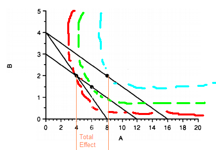
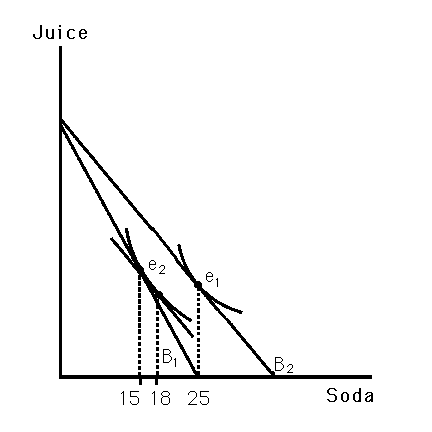
Remember: whenever the price of one good drops, our real income (purchasing power) rises. For theory's sake, in order to isolate the substitution effect, we must change the budget line to reflect changing price ratios while keeping real income constant. In order to do this, we take the budget line and rotate it around the point where it originally intersects with it's original indifference curve.

We look at where this new, streched budget line is tangent to a greater indifference curve. The change in the quantity of product A is caused by the substituion effect: consumers substituting into the cheaper good to maximize total utility (reach a greater indifference curve).

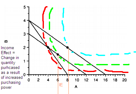
Now let's look at income effect: If total income increases when the price of a NORMAL GOOD decreases, that will also cause us to purchase more of that good. In order to look at the income effect, we take the restricted budget line (with the new price ratio) and shift it up and to the right to reflect the increase in real income.

The point where this new, inflated budget line is tangent to the highest indifference curve represents the new quantity purchased as a result of both substitution AND income effect.


Remember:
-The total effect is the substitution effect + the income effect
-The substitution is a change in quantity purchased due to a change in relative prices. It is always negative (except for conspicious consumption goods), which means that price and quantity purchased change in opposite directions
-Income effect is a change in quantity purchased due to a change in purchasing power.
It can be positive (for normal goods) or negative (for inferior goods)

If the income effect is greater than the substitution effect, the product in question is a Giffen Good


NOW: let's put it all together!

Indifference curve analysis yields the same conditions for total utility maximization as marginal utility analysis!

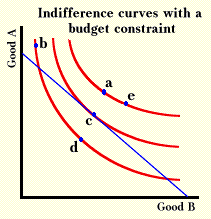
We know that for Utility to be maximized in indifference curve analysis, the budget line must be tangent to the indifference curve.

BUDGET LINE EQUATION: PxQx +PyQy = Income
BUDGET LINE SLOPE: -Px/Py (Marginal rate of tranformation)

INDIFFERENCE CURVE EQUATION: /\Qx(MUx) + /\Qy(MUy) = 0
INDIFFERENCE CURVE SLOPE: -MUx/MUy (Marginal rate of substitution)

Maximazation condition: The budget line must be tangent to the indifference curve

or

the slope of the budget line must equal the slope of the indifference curve

or

-Px/Py must = -MUx/MUy

or

MUx/Px = MUy/Py WHICH IS MARGINAL UTILITY ANALYSIS

Brilliant, non?

Econ 101 Indifference Curves:

Indifference curves are graphs which incorporate the idea of tastes or preferences.


We assume that consumers are rational thinkers, and that they can rank their preferences. There are three parts to this 'rationality':

1- COMPLETE the consumer must either prefer good A to good B, good B to good A, or be indifferent
2- REFLEXIVE A is always as good as A. Preferences don't change based on exogenous variables
3- TRANSITIVE If A > B and B > C, then A > C

THESE SUBJECTIVE PREFERENCES ARE INDEPENDANT (EXOGENOUS).
-We cannot make comparisons between different people (because you can't compare my happiness to yours)
-We cannot make comparisons between different times
-This shows us that psychology is the basis of microeconomics!

HOKAY! Now that the background stuff is out of the way, let's actually look at one of these again.

FUNCTION OF A UTILITY CURVE: U = U(x,y) higher number = higher utility...

All of the different points on one indifference curve show different combined quantities of 2 goods (x and y) which yield a constant total utility.
Because the utility derived from any product is different for different people, the indifference curve shows PERSONAL PREFERENCES.

CHARACTERISTICS:
For any two products, there are an infinite number of indifference curves expanding outward. The total utility for each progressive curve is higher than the last one, because each progressive curve represents a greater combined quantity of goods x and y, and in most cases, we prefer to have MORE (more goods = greater total utility).

Two indifference curves for the same product cannot cross, because that would suggest that we can achieve the same total utility with a set combination of x and y as we could with the same quantity of x, but fewer of y. Also the point of intersection would imply two different total utilities for the same combination of goods. That's illogical.

EQUATION: Change in X (Marginal utility of X) + Change in Y (Marginal utility of Y) = 0

Why? Because if two points are on the same indifference curve, the utility lost on one axis is gained on the other axis.

utility lost = Change in X (Marginal utility of X)
utility gained = Change in Y (Marginal utility of Y)

The slope of the indifference curve = change in X/change in Y

OR

negative marginal utility of X/marginal utility of Y

OR

the marginal rate of substitution!

COMBINING BUDGET LINES AND INDIFFERENCE CURVES:
both budget lines and indifference curves have the same axes: quantities of different products. Budget lines show us possible combinations of different products, and indifference curve show us desired combinations of different products!

REMEMBER, price changes are represented as rotations or stretches of the budget line. SO, if the price of soda falls, the budget line for soda stretches out further along the x-axis, and the possible quantity of soda increases. Consumers want to maximize total utility, so places where the indifference line meets the budget line represent the demanded combinations of goods, given the prices of both products. As the prices of a good falls, consumers substitute into that good in order to reach higher indifference curves with the stretched budget line.
.
In this way, we can see the formation of a demand curve- consumers buy greater quantities of a product as the price decreases in order to maximize total utility (intersect with the highest indifference curve). This results in a negatively sloped demand curve.

-------------

ECON 101: The beginning of consumer behavior

WE ARE STARTING TO LOOK AT CONSUMER BEHAVIOR!

Isn't it exciting!? In order to nicely coordinate with the way the midterm is working out, we are going to spread this unit out over a period of two weeks. The online test won't pop up until the 16th.

An interesting note: Prof Gateman thinks that population growth is the reason behind all of the world's problems.

OKAY! For this unit, we are going BEHIND the demand curve to discover what the psychological link is between consumer behavior and HAPPINESS

For instance, we will discover why the demand of a Louis Vitton Purse increases when the price increases. Sounds crazy? It might be, but it works, and we're going to find out why!

--------------
WE'RE STARTING WITH MARGINAL UTILITY ANALYSIS

In order to add up total demand for any specific product, we set the price for the product and then add up the quantity each individual consumer demands at that price (ceteris paribus) to find the total. The total market demand is the sum of each individual household's demand for the product!

Super-easy, right?

Total demand + total supply = An economy, but we don't get to total supply until next chapter...

See, there is a chain of 'bigness'

Individual consumer preferences make up household demand
Total household demand makes up market demand
Market demand plus market supply makes up an economy
An economy is awesome and interesting

In the mean while, we need to come to understand the basis for that demand at the individual consumer level.

HOKAY, now for the juicy stuff: MARGINAL UTILITY THEORY

Utility: We define utility as satisfaction, happiness, fulfillment of a want. Sometimes utility is also used as a method ranking products, or illustrating personal preferences.

Utility is an ORDINAL MEASURE (which means that we can rank utility, but unlike a cardinal measure, we cannot assign specific numeric value to it)

TOTAL UTILITY is the total satisfaction derived from consuming all units of the good (for instance, the total amount of satisfaction I derive from chugging 10 bottles of beer)

MARGINAL (extra, or incremental) UTILITY is the change in total utility which occurs as a result of consuming one additional unit of the good (ie, the amount of satisfaction I derive from chugging the 10th bottle of beer)

There is this thing in economics, and it is known as the
LAW OF DIMINISHING MARGINAL UTILITY
What it means is that marginal utility decreases as we continue to consume a certain product AFTER A CERTAIN POINT (ceteris paribus)

SEE!?

Why does this happen?
Well, it's because of opportunity cost. Usually, consumers are willing to give up more for the first quantity of a product than the for the 39th quantity of a product. A good example here is water. We would give up a LOT in order to have use of at least 1 litre of water per day. We would give up a significantly smaller amount to have use of 390 litres of water per day.

The FORMULAS:
Marginal Utility = (Change in Total Utility)/(Change in Quantity)
Marginal Utility is a derivative of total utility with regard to quantity

Total utility = The sum of the marginal utilities
Total utility is an integral of marginal utility

Let's review:
-Total utilty increases as a decreasing rate after a certain point (ceteris paribus)
-Marginal utility is the change in total utility divided by the change in quantity
-The slope of a line between two points on a total utility curve is the marginal utility of that product for that change in quantity
-Generally, total utility curve is S-shaped

The point where marginal utility stops increasing and begins to decrease is the inflexion point.
The reason why marginal utlity rises up to the inflexion point is that usually, the first bit of a product makes you crave or require even more of it (it's psychological).

After the inflexion point, total utility can still increase, but at a decreasing rate.

So... what can we do with this knowledge?

WELL we can try and maximize our utility, given two different products at different prices.

IN ECONOMICS, WE ALWAYS ASSUME THAT INDIVIDUALS SEEK TO MAXIMIZE THEIR TOTAL UTILITY. (We call this maximization principle). Individuals prefer happiness to unhappiness.

We will prove that individuals allocate income such that the utilty gained from the last dollar spent on each good is equal. In other words, that marginal utility per price on each good is equal. This can be expressed as an equation.

(marginal utility of product 1)/(Price of Product 1) = (Marginal utility of product 2)/(Price of product 2)

WE MAXIMIZE THE TOTAL UTILITY BY EQUATING THE MARGINAL UTILITIES.

Why do we use 'per dollar' utility? Because utility gained from one very expensive product is going to be much higher than utility gained from one cheap product, so we have to accomodate for that.
In these equations, we always assume that there is no utility gained by holding on to money (unless the money is considered a good, like in currency exchange scenarios)

So just think about that for a little while...

ECON 101 - Currency exchange, and excise taxes

Today, we're looking at two different applications of supply and demand: Currency Exchange, and Excise Taxes!

CURRENCY EXCHANGE:

The exchange rate is the price of a foreign currency in terms of a domestic currency. For an example, if 1 Canadian Dollar is Worth 2 British Pounds, the exchange rate of the British Pound is 2 Canadian Dollars.

The external value is the price of a domestic currency in terms of a foreign currency. For an example, if 1 Canadian Dollar is Worth 2 British Pounds, the external value of the Canadian Dollar is half a British Pound.

A good way to remember this is to remember that external value is 'all about me', so it's all about how much MY money is worth.

It's important to note that many major news sources don't always use these terms correctly.

OKAY! So why would people want to exchange currencies in the first place???

WELL, there two reasons.
1: They have a demand for foreign goods (so they need to convert their own currency into foreign currency in order to purchase them)
2: They want to make investments in foreign markets

SO...

Because of this, demand and supply of certain currencies depend on two factors.

DEMAND for a domestic currency depends on:
1- Demand for domestic exports
2- Foreign investment in domestic markets (K inflow)

SUPPLY of a domestic currency depends on:
1- Demand for foreign imports
2- Domestic investment in foreign markets (K outflow)

Let's say we're exchanging Canadian dollars for any kind of foreign currency. If the demand for Canadian dollars = the supply of Canadian dollars, we have EQUILIBRIUM

Things that can effect our dollar value:
-An increase in demand for Canadian goods
-A decrease in our own demand for foreign goods (in other words, a decrease in the supply of the Canadian dollar).

In this way, trade affects the currency market.

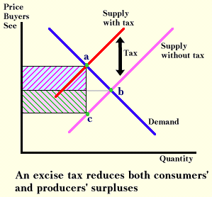
EXCISE TAXES: Basically, a sales tax which only applies to a specific item (carbon taxes, or sin taxes are examples of excise taxes)

There are two different kinds of excise taxes!
1: "AD VALOREM" ---> A percentage of the value of the product (like jewelry, slot machines, and matches)
2: "SPECIFIC" -------> A per-unit tax (quantity based) (like beer and cigarettes)

Also governments are considering creating an excise tax for fast food or trans fats... which could be interesting. The question is, does this tax serve as an effective disincentive?

TAX INCIDENCE is on whom the ultimate burden of a tax lies (aka: what percentage of the tax is paid for by consumers in the form of increased prices, and what percentage is paid for by the producer in the form of lost profits)

Basically, if you want to graphically introduce an excise tax, make a new supply curve above the original supply curve by the number of price units equal to the excise tax. Using this new curve, find the new equilibrium (where it intersects with demand at this new price). At this new quantity, the difference between the equilibrium price and the consumer price determines the consumer tax incidence, and the difference between the equilibrium price and the producer price determines the consumer tax incidence.

You can also manipulate the formulas for the curves using simple addition on the supply curve equal to the tax increase.

As a good rule of thumb, whichever curve (supply or demand) which is more inelastic will bear the majority of the tax incidence.

HOKAY! WHAT HAVE WE LEARNED SO FAR!?

Government intervention has a cost! It requires alternative allocation mechanisms, and generally the free market is much more efficient.

The free market can be a cruel cruel place...

but goddammit, it works!


An excise tax functions like an effect cost increase, and as such, it shifts the supply curve left for any product.
The consumer price = the producer price + the tax